The Dataset Is the Input
How prior-data fitted networks learn from synthetic worlds and make predictions on new datasets without task-specific weight updates.
On this page
- A CSV is not automatically a prediction model
- The idea has a long history
- Build worlds. Hide answers. Repeat.
- What the network learns to approximate
- TabPFN makes the dataset part of the input
- Time has to enter through the representation
- SAP and Nvidia have noticed the database
- What becomes easier, and what remains your job
- Footnotes
PFNs, synthetic worlds, and why the next useful foundation model might spend its life looking at your database.
In the space of ten weeks this summer, two of the largest companies in enterprise computing bought small labs that do not build chatbots. SAP agreed to acquire Prior Labs, the Freiburg team behind TabPFN, in May and closed the deal in July with a commitment of more than €1 billion over four years. Nvidia’s acquisition of Kumo AI, the company behind a relational foundation model, was reported in June.12
Neither company was short of language models. What they bought was a different bet: that the most valuable prediction problems in a business live in tables, and that a model can be pretrained to learn those problems from the examples you hand it.
That bet is worth understanding, because it cuts against the habit of the last three years. Give an LLM a spreadsheet and ask which customers will leave next month. It can explain churn, suggest features, write the SQL, and produce a confident paragraph about engagement. Ask it for reliable probabilities on customers it has never seen, and you have a different engineering problem. A forecast comes with decimal places, so it looks as though somebody did the mathematics.
The alternative is to pretrain a model specifically to learn a prediction problem from the examples we give it. That is the idea behind Prior-data Fitted Networks, or PFNs: train across many generated learning problems, then use the resulting network to make predictions on a new dataset. The new dataset changes the model’s predictions without changing its weights.3
The learning problem itself becomes an input.
A CSV is not automatically a prediction model
A table carries more structure than its text serialization suggests. Columns have types, scales, missing values, and relationships. Rows might represent independent customers, repeated measurements of the same person, or successive moments in time. The same numbers require different treatment in each case.
A general chat LLM can help interpret that structure. It can call Python, train a conventional model, and explain the results. But a system that uses an LLM to operate a forecasting tool is different from one that relies on the LLM itself to estimate the forecast.
Research has tried to bridge this gap directly. Time-LLM, published at ICLR 2024, maps time-series patches into representations aligned with a frozen language model and adds contextual prefixes — a serious modeling approach, with learned components around the LLM.4
The results deserve scrutiny. In Are Language Models Actually Useful for Time Series Forecasting?, Tan and colleagues examined three LLM-based forecasting approaches. Removing the LLM, or replacing it with a basic attention layer, often preserved or improved performance. The expensive language backbone was not earning its place.5
That does not prove language can never improve forecasting. News, maintenance notes, and known business events carry information a numerical history lacks. It does mean we should test which component contributes the gain, or we end up building an elaborate adapter and crediting whatever famous model sits behind it.
Compare Chronos. It uses language-model architectures, but its training procedure scales and quantizes numerical series into tokens and trains on real and synthetic time-series data. Its objective is forecasting from numerical histories. It is not a chatbot persuaded to become an accountant.6
The lesson: choose the training objective and data representation for the prediction problem. A transformer architecture does not make every model an LLM.
The idea has a long history
“Learning to learn” has been a research ambition for decades. Early meta-learning work includes Schmidhuber’s 1987 thesis. By 2016, Andrychowicz and colleagues were learning an optimizer that could update another model. In 2017, Model-Agnostic Meta-Learning (MAML) trained models toward an initialization from which a few gradient steps could adapt them to a new task.789
These approaches share an ambition — experience across tasks should make the next task easier — but they adapt differently. A learned optimizer still updates parameters. MAML prepares parameters for rapid fine-tuning. A PFN performs adaptation through the examples supplied in its input.
The PFN work appeared as a preprint in December 2021 and was published at ICLR 2022 as Transformers Can Do Bayesian Inference. Müller, Hollmann, Pineda Arango, Grabocka, and Hutter showed how training on sampled tasks could teach a network to approximate Bayesian prediction.3
TabPFN followed with a 2022 preprint and an ICLR 2023 paper, applying the approach to small tabular classification. The 2025 Nature paper expanded the case with classification and regression results on larger, more varied datasets.1011
So machines have not suddenly acquired the ability to learn how to learn. What has changed is that this research direction has become a useful, increasingly accessible option for ordinary prediction workloads — and, as of this summer, a strategically expensive one.
Build worlds. Hide answers. Repeat.
Imagine teaching someone to infer an unfamiliar rule. You could give them a thousand examples governed by the same rule; they would become good at that one problem. Or you could repeatedly change the rule, show a few examples, and ask them to predict what comes next.
In one exercise the answer depends on a linear relationship. In another, a threshold. In a third, two variables interact. Some exercises contain noise; others contain irrelevant inputs. To keep succeeding, the learner must use the examples to work out which kind of problem it is facing.
This is PFN pretraining, simplified. Researchers specify a prior distribution over tasks: a generator that defines which data-generating processes are possible and how often they appear. They sample a task, generate labeled examples, hide some answers, and train the network to predict them from the rest. Then they sample another task.3
“Synthetic worlds” is a useful metaphor for those sampled processes. A world need not simulate a bank, hospital, or school. It can be a mathematical mechanism that produces inputs and outcomes:
| Generated world | Example hidden rule | What the exercise demands |
|---|---|---|
| Linear | The target is a weighted sum of inputs | Infer direction and scale |
| Threshold | The outcome changes beyond a boundary | Locate the boundary from evidence |
| Interaction | Two inputs matter jointly | Detect a relationship a single column misses |
| Noisy | Identical inputs can have different outcomes | Represent uncertainty |
| Distracted | Most columns do not affect the target | Resist irrelevant information |
These are illustrative; actual priors are richer. The original TabPFN prior included structural causal models, with a preference for simpler structures.10
Generating tasks is different from generating rows. Random rows without a coherent relationship offer little to learn. Repeating one relationship teaches that relationship. Sampling diverse mechanisms creates a curriculum in which inferring the relationship is repeatedly necessary.
The generator also exposes the assumptions. Which relationships are common? How much noise is plausible? How often should a simple explanation be preferred? Those decisions shape what the network learns to expect. The synthetic-data factory is part of the model’s design, even if it never appears in the inference API.
This is why prior design has become its own research problem. Mitra, for example, studies mixtures of synthetic priors and how their diversity affects tabular generalization. The question has moved from whether we can manufacture training data to which manufactured learning problems teach useful habits.12
What the network learns to approximate
Suppose our observed dataset is , and we want the outcome for a new input . Bayesian prediction considers possible explanations of the observations and combines their predictions according to how plausible each explanation remains:
Here describes a possible underlying mechanism. Computing this integral is usually hard. PFNs approximate the resulting predictive distribution directly: the pretraining loss rewards assigning high probability to held-out answers across sampled datasets, and under the objective’s theoretical conditions its optimum is the posterior predictive distribution for the chosen prior.3
This lets us spend compute ahead of time to make future inference cheap. The term is amortized inference: spread the cost of learning an inference procedure across many later problems. A 2025 position paper frames exactly this opportunity, especially where real observations are expensive to acquire.13
“For the chosen prior” carries a lot of weight. The network is finite, training is finite, and the real dataset may differ from the generated tasks. Nagler’s statistical analysis makes clear that generalization depends on properties of the predictor; the PFN label is not an accuracy guarantee.14
I find this more compelling than treating synthetic data as an unlimited substitute for reality. It is a specific way to transfer assumptions and computational effort into a new prediction problem. Whether those assumptions help remains an empirical question.
TabPFN makes the dataset part of the input
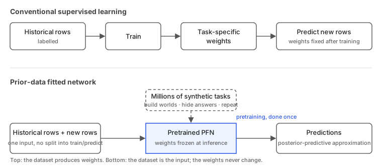
In ordinary supervised learning, we fit a model on historical examples, obtain task-specific parameters, and use those parameters to predict new cases. With a pretrained TabPFN, labeled historical examples and the new cases are supplied together to a network that already learned across many tasks. It conditions on those examples without another round of weight updates.10
This is in-context learning. “Training data” still exists, but it serves as inference-time context. The library keeps the familiar interface, which makes the procedure look more conventional than it is:15
from tabpfn import TabPFNClassifier
clf = TabPFNClassifier()clf.fit(X_history, y_history)      # no gradient steps: the rows become contextproba = clf.predict_proba(X_new)   # probabilities for cases the model has never seen
Nothing in fit learns weights. It stores and preprocesses the examples; the learning happens inside predict_proba, every time.
Suppose a business has a few hundred completed support tickets and wants to predict whether a new ticket will breach its resolution deadline. Inputs might include queue, issue category, initial severity, workload at creation, and customer history available at that moment. Known outcomes on earlier tickets provide examples of the local relationship. A new ticket supplies the query.
Whether TabPFN wins on that task needs testing. The change is that trying it no longer requires training a deep network from scratch on a few hundred rows.
The 2025 Nature evaluation established strong results in the small-to-medium regime, including datasets with up to 10,000 samples and 500 features. The May 2026 TabPFN-3 technical report claims scaling to one million training rows and improved performance across several benchmark families — author-reported results under specific hardware and evaluation conditions.1116
TabPFN is the prominent implementation, not the whole category. TabICL and Mitra, among others, pursue the same idea.1712
Time has to enter through the representation
A tabular learner cannot recover temporal information the input has discarded. Two students can have the same average score while one is improving and the other declining. Two machines can have the same average temperature while one spikes harmlessly and the other is steadily overheating.
For a longitudinal problem we still need a representation of history: trends, recency, changes between windows, calendar features, or a learned state summarizing the sequence. An encoder followed by a PFN is a reasonable architecture. There is already a concrete forecasting example: TabPFN-TS combines the pretrained TabPFN-v2 with lightweight temporal features and treats forecasting as tabular regression, with no time-series-specific pretraining.18
This is also why “zero-shot forecasting” confuses readers. It means no task-specific parameter training. Historical observations still enter the model as context; the model has not become independent of evidence.
My working position is that a learned history encoder earns its place only by passing two tests, and most published comparisons run neither properly.
The first is a loss-of-signal test. When an entity’s history is wider than what fits in a tabular model’s context — hundreds of events per customer, years of readings per machine — something has to compress it. The question is whether the compressed representation keeps the evidence that actually mattered, or whether it keeps whatever was easiest to summarize. The honest comparison is against a model that saw the full history by other means, not against a model that saw nothing.
The second is a beat-the-analyst test. A competent analyst can write lags, rolling means, days-since-last-event, and trend slopes in an afternoon. If a learned encoder only beats a deliberately weak feature set, nothing has been learned about the encoder. It has to beat the afternoon’s work, on later periods, with the same tabular model downstream.
Run both against a seasonal baseline and an established forecasting method, and evaluate on time-based splits. That is the bar I hold my own experiments to, and I would not trust a temporal-plus-PFN result that does not report it.
SAP and Nvidia have noticed the database
The two acquisitions address related opportunities, but the models should not be collapsed into one explanation.
The classic TabPFN setup operates on a flat table. KumoRFM addresses connected relational data: customers linked to orders, orders to products, products to categories, with timestamps and additional relationships carrying predictive information. It combines row encoding, a relational graph transformer, and in-context examples, and its pretraining uses public real-world databases as well as synthetic relational data. The KumoRFM-2 preprint extends the direction with scaling and further relational evaluations.1920
Consider churn prediction. An order count and a “days since last purchase” column might be useful, but the evidence could also sit in returns, support interactions, changing purchase patterns, or connections to particular products. A relational model can work with those connected records instead of requiring every relationship to be manually compressed into one feature table.
My reading is that structured prediction has become strategically valuable to large platform companies because enterprise databases contain questions with measurable consequences: demand, delays, failures, recommendations, customer behavior. SAP’s €1 billion is an investment plan, not the acquisition price, and neither deal is evidence that either model wins every benchmark. An acquisition announcement cannot substitute for your test set.
What becomes easier, and what remains your job
These models are most interesting when a useful supervised problem exists but building and maintaining a separate pipeline for every variation is expensive. Small scientific experiments, operational risk estimates, lead scoring, and equipment failure prediction all qualify. Relational models broaden the scope to questions whose evidence spans connected tables.
Education shows both the opportunity and the boundary. Given assessment history and reliable outcomes, a model might estimate the likelihood of a student struggling with a particular concept, which helps prioritize attention. It does not identify which lesson plan will cause the greatest improvement. Predicting an outcome and estimating the effect of an intervention require different evidence.
The cold-start promise needs the same precision. PFNs reduce the burden of fitting a task from limited examples by bringing a pretrained inference procedure to it. They cannot manufacture trustworthy local labels, reveal an unmeasured variable, or prove that a synthetic learning process matches a real classroom.
For an engineer, the work shifts toward defining the task well. Decide exactly what is being predicted, over which horizon, using which information is available at prediction time. Compare against strong conventional baselines. For temporal data, evaluate on later periods; for repeated entities, split to match the intended deployment. Check whether the probability estimates are useful for the decision being made, rather than admiring accuracy in isolation.
And price the whole system. Avoiding task-specific training does not make inference free. Context processing, GPU memory, repeated predictions, preprocessing, and serving constraints still decide whether a model belongs in production.
What interests me most is bringing good prediction to problems too small to justify their own ML project. A team might have enough evidence to make a useful estimate but not the time or expertise to build another pipeline. A pretrained learner lowers that threshold.
The familiar workflow asks us to collect a dataset and train a model for it. PFNs introduce another option: collect a dataset and give it to a model that has already practiced learning across many possible datasets.
That is a meaningful change. Its value will show up in the next unfamiliar problem we can solve with the evidence we actually have.
References and further reading
Research dates distinguish preprints from conference publication where relevant. Acquisition details checked on October 10, 2026. Numerical results are attributed to their specific publications; application scenarios are illustrations, not claims of deployments or measured performance.
Footnotes
-
SAP, SAP to Acquire Prior Labs, May 4, 2026, and SAP Completes Acquisition of Prior Labs, July 17, 2026. The latter states the planned investment of more than €1 billion over four years. ↩
-
Sharon Goldman, Nvidia snaps up Kumo AI in latest acquisition, Fortune, June 3, 2026. Terms were not disclosed by either company; The Information separately reported a figure above $400 million. Used for the transaction report, not technical claims. ↩
-
Samuel Müller, Noah Hollmann, Sebastian Pineda Arango, Josif Grabocka, and Frank Hutter, Transformers Can Do Bayesian Inference, preprint 2021; ICLR 2022. The PFN training objective and posterior-predictive interpretation. ↩ ↩2 ↩3 ↩4
-
Ming Jin et al., Time-LLM: Time Series Forecasting by Reprogramming Large Language Models, preprint 2023; ICLR 2024. ↩
-
Mingtian Tan, Mike A. Merrill, Vinayak Gupta, Tim Althoff, and Thomas Hartvigsen, Are Language Models Actually Useful for Time Series Forecasting?, NeurIPS 2024. Ablations of three LLM-based approaches. ↩
-
Abdul Fatir Ansari et al., Chronos: Learning the Language of Time Series, TMLR 2024. ↩
-
Jürgen Schmidhuber, 1987 thesis on learning how to learn. An early historical example, linked through the author’s archive. ↩
-
Marcin Andrychowicz et al., Learning to learn by gradient descent by gradient descent, NeurIPS 2016. ↩
-
Chelsea Finn, Pieter Abbeel, and Sergey Levine, Model-Agnostic Meta-Learning for Fast Adaptation of Deep Networks, ICML 2017. ↩
-
Noah Hollmann, Samuel Müller, Katharina Eggensperger, and Frank Hutter, TabPFN: A Transformer That Solves Small Tabular Classification Problems in a Second, preprint 2022; ICLR 2023. ↩ ↩2 ↩3
-
Noah Hollmann et al., Accurate predictions on small data with a tabular foundation model, Nature 637, 319–326, 2025. Classification, regression, synthetic priors, and the TabPFN-v2 evaluation. ↩ ↩2
-
Xiyuan Zhang et al., Mitra: Mixed Synthetic Priors for Enhancing Tabular Foundation Models, 2025. ↩ ↩2
-
Samuel Müller et al., Position: The Future of Bayesian Prediction Is Prior-Fitted, ICML 2025 position paper. ↩
-
Thomas Nagler, Statistical Foundations of Prior-Data Fitted Networks, ICML 2023. ↩
-
Prior Labs, official TabPFN implementation. The snippet above follows the v2 interface; check the repository for release-specific details. ↩
-
Léo Grinsztajn et al., TabPFN-3: Technical Report, May 2026. Author-reported scaling and benchmarks; distinct from the peer-reviewed 2025 Nature evaluation. ↩
-
Jingang Qu et al., TabICL: A Tabular Foundation Model for In-Context Learning on Large Data, 2025. ↩
-
Shi Bin Hoo, Samuel Müller, David Salinas, and Frank Hutter, From Tables to Time: Extending TabPFN-v2 to Time Series Forecasting, posted 2025; revised January 2026. ↩
-
NVIDIA, KumoRFM: A Relational Foundation Model. Official documentation on relational encoding, pretraining sources, and in-context prediction. ↩
-
Valter Hudovernik et al., KumoRFM-2: Scaling Foundation Models for Relational Learning, April 2026. ↩
LogCTL Dispatch
New essays, experiments and workflows. No daily noise.
Usually 2–4 emails a month.
Comments
Loading comments…